Does the autumn ENSO state predict a wet Front Range winter? This cookbook answers that one classification question on NSF NCAR’s CESM2 Large Ensemble, following NSF Unidata’s Supervised Machine Learning Readiness. This chapter frames the question and finds the data.
Code: Apache-2.0 · Content: CC BY 4.0 · Data: NCAR CESM2 Large Ensemble Cloud-Optimized Dataset (Grover & Banihirwe 2021, doi:10.26024/y48t-q717) and Rodgers et al. 2021 (doi:10.5194/esd-12-1393-2021), UCAR Data Terms of Use; Community Earth System Model v2 Large Ensemble (CESM2 LENS) was accessed on 2026-10-20 from https://
Drafted with AI assistance (Anthropic’s Claude) from cited sources, under the author’s direction, and reviewed by the author in several full read-throughs.
Text and code were checked against those sources and the notebooks’ own outputs by the author’s automated checks (not in this repository) and by separate AI review sessions (also Claude); no human subject-matter expert has reviewed it yet.
Overview¶
A classifier will read one number, a member’s autumn Niño 3.4 state, and say whether that member’s coming Front Range winter will be
wet. This chapter frames that question as a decision, finds the data in the intake-esm catalogue, records it in a Metadata
Document, and loads the committed table.
The spine is Unidata’s (Apache-2.0), except that the split is by ensemble member (chapter 3). Terms are in the
glossary; shared code is in lensml.py, and show() prints a function’s source.
Prerequisites¶
| Concepts | Importance | Notes |
|---|---|---|
| Pythia Foundations: Introduction to Xarray | Necessary | a Zarr store, a box selection, groupby |
| Xarray tutorial | Helpful | the same ground, in more depth |
| Intake-ESM | Helpful | one catalogue search |
| scikit-learn | Not required | every call is introduced where it is used |
Time to learn: about 15 minutes with the Try it boxes. Cells run in seconds from the committed cache; the catalogue cells need a network route to AWS.
System requirements: the
environment.ymlat the repository root; no account, no local data beyond the committed cache.
Imports¶
The second cell prints the package versions; one that disagrees with environment.yml means the wrong kernel.
import importlib.metadata
import os
import re
import sys
from datetime import datetime

import intake
import matplotlib.pyplot as plt
import numpy as np
import pandas as pd
import xarray as xr
from lensml import (
    FRONT_RANGE,
    NINO34,
    PARAMS_RECORD,
    SEASON,
    credit_own,
    derive_member_winters,
    load_cache,
    show,
    show_fig,
)
now = datetime.now().astimezone().isoformat(timespec="seconds")
print(f"run started {now} kernel python {sys.version.split()[0]}")
PACKAGES = [
"numpy",
"pandas",
"scipy",
"scikit-learn",
"matplotlib",
"xarray",
"zarr",
"s3fs",
"cftime",
"intake",
"intake-esm",
]
for pkg in PACKAGES:
try:
print(f"{pkg:13s} {importlib.metadata.version(pkg)}")
except importlib.metadata.PackageNotFoundError:
print(f"{pkg:13s} NOT INSTALLED: re-create the environment")run started 2026-10-30T21:55:56+00:00 kernel python 3.12.16
numpy 2.5.4
pandas 3.0.6
scipy 1.18.1
scikit-learn 1.9.1
matplotlib 3.11.2
xarray 2026.9.0
zarr 3.4.2
s3fs 2026.9.0
cftime 1.6.5
intake 2.0.9
intake-esm 2025.12.12
The question, as a decision¶
The person who acts on the answer is a forecaster drafting a local winter-outlook briefing, such as NWS Boulder’s (2020) or NWS Pueblo’s (2025). The SON mean is complete only on 30 November, so this input serves a December update at zero lead; those two briefings date, by their files, from mid-September and mid-October, before it exists, and would need an earlier input (JJA for Boulder’s, JAS for Pueblo’s: a parameter edit and a rebuild). Pueblo’s briefing relays the Climate Prediction Center’s official lean and reports what the ENSO state statistically suggests locally. A “wet” call right more often than the base rate, without missing most wet winters, would be the precondition for testing that on observed winters (every score here is CESM2 against CESM2), beside CPC’s “equal chances”, as Pueblo’s 2025 briefing did for southeast Colorado, mostly south of the box: “Statistically, warmer and drier SE CO, but CPC’s forecast is equal chances …”.
Every parameter in lensml.py is a design decision with its reason; changing one is a trial you record. The seed is declared once and
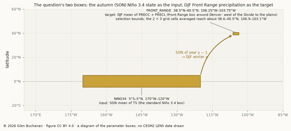
passed down, never np.random.seed() (scikit-learn’s Common pitfalls, §12.3.3). The figure draws the two boxes from those
parameters.
def span(box):
    """A box as degrees with hemispheres, from its slices on the 0-360 grid."""
    y0, y1 = box["lat"].start, box["lat"].stop
    x0, x1 = box["lon"].start, box["lon"].stop

    def lat(y):
        return f"{abs(y):g}°{'S' if y < 0 else 'N'}"

    def lon(x):
        return f"{x:g}°E" if x <= 180 else f"{360 - x:g}°W"

    return f"{lat(y0)}–{lat(y1)}, {lon(x0)}–{lon(x1)}"


fig, ax = plt.subplots(figsize=(9, 3.8))
ax.set(xlim=(165, 275), ylim=(-24, 56), ylabel="latitude")
ax.set_title(
    "The question's two boxes: the autumn (SON) Niño 3.4 state as the input, "
    f"{SEASON} Front Range precipitation as the target",
    fontsize=9,
)
xt = list(range(170, 276, 15))
ax.set_xticks(xt)
ax.set_xticklabels(
    [f"{x}°E" if x <= 180 else f"{360 - x}°W" for x in xt], fontsize=8
)
yt = list(range(-20, 61, 20))
ax.set_yticks(yt)
ax.set_yticklabels(
    [f"{abs(y)}°{'S' if y < 0 else 'N'}" for y in yt], fontsize=8
)
ax.axhline(0, lw=0.8, c="#6A7077", ls=":")
ax.grid(True, lw=0.5)
boxes = [
    (
        "NINO34",
        NINO34,
        "input: SON mean of TS (the standard Niño 3.4 box)",
        (215, -13),
        "top",
    ),
    (
        "FRONT_RANGE",
        FRONT_RANGE,
        f"target: {SEASON} mean of PRECC + PRECL (Front Range box around Denver: "
        "west of the Divide to the plains)\nselection bounds; the 2 × 3 grid cells averaged reach about "
        "38.6–40.5°N, 106.9–103.1°W",
        (236, 50),
        "bottom",
    ),
]
for name, box, note, at, va in boxes:
    x0, x1 = box["lon"].start, box["lon"].stop
    y0, y1 = box["lat"].start, box["lat"].stop
    ax.add_patch(
        plt.Rectangle(
            (x0, y0),
            x1 - x0,
            y1 - y0,
            facecolor="#C9A23A",
            edgecolor="#8F7022",
            lw=1.2,
            zorder=3,
        )
    )
    ax.annotate(
        f"{name}  {span(box)}\n{note}",
        xy=((x0 + x1) / 2, y0 if va == "top" else y1),
        xytext=at,
        fontsize=7.5,
        ha="center",
        va=va,
        arrowprops=dict(arrowstyle="-", color="#6A7077", lw=0.8),
    )
ax.annotate(
    "",
    xy=(FRONT_RANGE["lon"].start, FRONT_RANGE["lat"].start),
    xytext=(NINO34["lon"].stop, NINO34["lat"].stop),
    arrowprops=dict(
        arrowstyle="->",
        color="#8F7022",
        lw=1.6,
        connectionstyle="arc3,rad=-0.25",
    ),
)
ax.text(
    243,
    22,
    f"SON of year y − 1\n→ {SEASON} winter y",
    fontsize=8,
    ha="right",
    va="center",
    color="#8F7022",
)
credit_own(fig, "a diagram of the parameter boxes; no CESM2 LENS data drawn")
plt.tight_layout()
show_fig(
    fig,
    (
        "Schematic map on a longitude–latitude frame with no coastlines: "
        "a wide gold rectangle on the equator marks the Niño 3.4 box "
        "(5°S–5°N, 170°–120°W) over which the autumn input is averaged; a"
        " small gold rectangle near 39.5°N, 105°W marks the Front Range "
        "box over which the winter precipitation target is averaged; a "
        "curved arrow from the first to the second is labelled with the "
        "season step from the autumn of one year to the following winter."
    ),
)
Framing: Unidata’s three questions¶
Unidata opens every analysis with three questions, so that the target answers someone’s decision.
The worked answers
Does a simpler solution exist? Three, and a model is measured against them, not assumed to beat them.
| Simple solution | What it predicts | What it sets |
|---|---|---|
| always-dry | “dry” every winter | a bar on accuracy only (wet precision and recall are 0) |
| always-wet | “wet” every winter | recall 1 at precision = the base rate: the bar every precision is read against |
| Niño-sign rule | “wet” when the autumn Niño 3.4 anomaly is positive | the physical prior (NWS Boulder east of the Divide: El Niño wetter, La Niña drier); no bar |
Can machine learning requirements be met? On the data side, yes: the catalogue holds monthly PRECC, PRECL and TS for every historical member in both forcing variants. On the physics side the honest prior is a small effect: Stagge et al. (2023) find the ENSO winter-precipitation signal over the Intermountain West is a north–south dipole, “the northern pole … north of 40° N” and “the southern pole remains south of 35° N, with some northward creep along the eastern edge of the study area”. The Front Range (about 38.5–40.5° N), in the eastern part of their area, sits mostly between them by latitude, its northern edge just past 40° N, and the northern pole’s sign reversed (La Niña wetter). Their map of the effect in millimetres (Fig. 1b) is finer: it shades Colorado’s central mountains, which the box’s west column partly covers, with the northern pole’s sign (wetter under La Niña, drier under strong El Niño), so the box mixes two priors. The signal is measured here, not assumed.
Which scientific question should be answered? Given the autumn Niño 3.4 state in a CESM2 LENS member, will that member’s coming Front Range winter be wet — above the one pooled threshold that marks the upper third of the training members’ detrended winters?
The catalogue on AWS¶
The catalogue forces two design facts: there is no monthly PRECT, so the target is PRECC + PRECL; and there is no variable
named SST, so the Niño 3.4 index is built from atmospheric TS over open ocean. The first cell lists the six stores; the second
computes what a box subset reads. Offline, each prints OFFLINE and the chapter runs from the cache.
CATALOG_URL = "https://ncar-cesm2-lens.s3-us-west-2.amazonaws.com/catalogs/aws-cesm2-le.json"
try:
    cat = intake.open_esm_datastore(CATALOG_URL)
    subset = cat.search(
        component="atm",
        frequency="monthly",
        experiment="historical",
        variable=["PRECC", "PRECL", "TS"],
    )
    print(
        f"catalogue last_updated: {cat.esmcat.last_updated}   "
        f"rows in catalogue: {len(cat.df)}   rows selected: {len(subset.df)}"
    )
    cols = [
        "variable",
        "forcing_variant",
        "units",
        "start_time",
        "end_time",
        "path",
    ]
    with pd.option_context(
        "display.max_colwidth", None
    ):  # the six paths in full
        display(subset.df[cols])
except Exception as err:  # no network, a DNS failure, S3 unreachable
    if os.environ.get("CI"):  # CI has network: a failure there is real
        raise
    cat = subset = None
    print(
        f"OFFLINE: the catalogue at {CATALOG_URL} could not be read "
        f"({type(err).__name__}). The Metadata Document's catalogue and store "
        "rows are *not printed this run*; every later cell runs from the cache."
    )
catalogue last_updated: 2021-12-27 14:29:25+00:00 rows in catalogue: 322 rows selected: 6
try:
    probe = xr.open_zarr(
        "s3://ncar-cesm2-lens/atm/monthly/cesm2LE-historical-cmip6-TS.zarr",
        consolidated=True,
        storage_options={"anon": True},
    )
except Exception as err:  # offline: the structure rows are not printed
    if os.environ.get("CI"):  # CI has network: a failure there is real
        raise
    probe = None
    print(
        f"OFFLINE: the TS store could not be opened ({type(err).__name__}); "
        "the dims, calendar and chunking rows are *not printed this run*."
    )
if probe is not None:
    print("dims      :", dict(probe.sizes))
    print("coords    :", list(probe.coords))
    print(
        "members   :",
        probe.member_id.values[:3],
        "…",
        "calendar:",
        type(probe.time.values[0]).__name__,
    )
    ch = tuple(int(c) for c in probe["TS"].encoding["chunks"])
    per_chunk = (
        int(np.prod(ch)) * probe["TS"].dtype.itemsize
    )  # bytes, uncompressed
    n_time_chunks = -(
        -probe.sizes["time"] // ch[1]
    )  # chunks along time per member
    per_member_var = n_time_chunks * per_chunk
    n_members = (
        2 * probe.member_id.size
    )  # two halves, each the size of this store
    print(
        f"chunking  : {ch} {probe['TS'].dtype} → {per_chunk / 1e6:.0f} MB per chunk "
        f"uncompressed; one member-variable ({probe.sizes['time']} months) = "
        f"{n_time_chunks} chunks × {per_chunk / 1e6:.0f} MB ≈ {per_member_var / 1e6:.0f} "
        f"MB read for any box subset; the derivation ({n_members} members × 3 "
        f"variables) ≈ {n_members * 3 * per_member_var / 1e9:.0f} GB"
    )
dims : {'member_id': 50, 'time': 1980, 'lat': 192, 'lon': 288, 'nbnd': 2}
coords : ['lat', 'lon', 'member_id', 'time', 'time_bnds']
members : ['r10i1181p1f1' 'r10i1231p1f1' 'r10i1251p1f1'] … calendar: DatetimeNoLeap
chunking : (1, 600, 192, 288) float32 → 133 MB per chunk uncompressed; one member-variable (1980 months) = 4 chunks × 133 MB ≈ 531 MB read for any box subset; the derivation (100 members × 3 variables) ≈ 159 GB
The Metadata Document¶
Unidata’s Metadata Document records the data in four parts (general, structure, quality, provenance), each row naming its evidence.
The three Quality rows carry into later chapters: the historical smbb half has no ocean TEMP, so both halves use TS; smbb also differs in
forcing (smoothed biomass burning, 1990–2020), so chapter 2 checks base rates per half; and members “should not be considered … independent” soon after
1850, so chapter 3 measures what independence is left by 1900.
The Metadata Document, row by row
| Part | Value | Evidence |
|---|---|---|
| General | CESM2 LENS on AWS Open Data, historical, 1850–2014; UCAR Data Terms of Use (CC BY 4.0): cite the DOI and the paper | registry |
| Structure | PRECC, PRECL, TS × forcing cmip6, smbb; ≈1°, monthly, noleap; PRECC/PRECL m/s → mm/day × 8.64e7; TS in K | catalogue paths; dims, members lines |
| Structure | two equal forcing halves; 20 micro-members per start year (four AMOC phases) | project page; Rodgers §2.2 |
| Structure | one row = one member-winter: SON Niño 3.4, season-mean Front Range PRECT | derive_member_winters |
| Quality | no historical ocean TEMP for smbb → TS for both halves | catalogue |
| Quality | smbb = smoothed biomass burning 1990–2020 + “two sets of bug corrections”; base rates per half (chapter 2) | project page |
| Quality | members “should not be considered … independent” soon after 1850, and Rodgers et al. analyse internal variability “after 1960”; the 1900 start rests on chapter 3’s sibling check, not on Rodgers | Rodgers §2.2 |
| Provenance | aws-cesm2-le.json, DOI 10.26024/y48t-q717; anonymous S3, us-west-2; ACCESS_DATE, asserted against the cache header | last_updated line; the cache cell |
The member-winter table¶
Two box means per member read the volume the chunking line computes, so the derivation runs once and writes
data/member_winters.csv for every chapter. Its reader asserts that the header records the current parameters and an access=
date equal to ACCESS_DATE (the cache header matches lensml.py line). The committed header predates AUTUMN_MONTHS; the reader
assumes SON and prints a line saying so.
show(derive_member_winters, load_cache)Rebuilding. REBUILD = True re-derives the table from S3: 33 minutes for the full ensemble on a fast link (2026-10-20), an
hour or more on home broadband; fewer members is a quick sample. A rebuild stamps its own access date (and AUTUMN_MONTHS) into the
header; the chapters then ask you to set ACCESS_DATE to match.
REBUILD = False  # True re-derives data/member_winters.csv from S3
N_MEMBERS_PER_HALF = (
    50  # used only when REBUILD = True; 50 = the full ensemble
)

table, cache_header, access_date = load_cache(REBUILD, N_MEMBERS_PER_HALF)
print(cache_header)
print(
    "cache header matches lensml.py:", PARAMS_RECORD, f"· access={access_date}"
)
n_header = 2 * int(
    re.search(r"n_members_per_half=(\d+)", cache_header).group(1)
)
n_store = (
    2 * probe.member_id.size if probe is not None else None
)  # unknown offline
if n_store:
    kind = (
        "A SAMPLE"
        if table.member_id.nunique() < n_store
        else "the full ensemble"
    )
    of_store = f"of {n_store} in the two stores ({kind})"
else:
    of_store = (
        f"(offline: the header says it was derived from {n_header} members)"
    )
print(
    f"{len(table)} member-winters · {table.member_id.nunique()} members {of_store} "
    f"· winters {table.winter.min()}–{table.winter.max()}"
)
table.head()
cache header has no AUTUMN_MONTHS field (it predates the field): taken as AUTUMN_MONTHS=[9, 10, 11], the only autumn the derivation code had: the file's autumn is assumed, not read from the header. A rebuild records it.
# derived by 02_applications.ipynb: SEASON=DJF WINDOW=(1900, 2014) FRONT_RANGE={'lat': slice(38.5, 40.5, None), 'lon': slice(253.75, 256.25, None)} NINO34={'lat': slice(-5, 5, None), 'lon': slice(190, 240, None)} n_members_per_half=50 RNG_SEED=0 access=2026-10-20
cache header matches lensml.py: SEASON=DJF WINDOW=(1900, 2014) FRONT_RANGE={'lat': slice(38.5, 40.5, None), 'lon': slice(253.75, 256.25, None)} NINO34={'lat': slice(-5, 5, None), 'lon': slice(190, 240, None)} AUTUMN_MONTHS=[9, 10, 11] · access=2026-10-20
11500 member-winters · 100 members of 100 in the two stores (the full ensemble) · winters 1900–2014
Summary¶
The question is a forecaster’s decision at the start of winter (the SON input completes on 30 November), measured against
three simple rules. The data are in a Metadata Document whose rows
point at printed evidence; the table is asserted against the parameters on every read (the cache header matches lensml.py line).
What’s next?¶
Chapter 2 explores the target and input, removes the forced response on the training members only, and defines “wet”.
Resources and references¶
| Resource | Where it bears | Licence |
|---|---|---|
| Grover, M., & Banihirwe, A. (2021). NCAR CESM2 Large Ensemble Cloud-Optimized Dataset. NSF NCAR CISL. doi:10.26024/y48t-q717 | the dataset (required citation) | UCAR Data Terms of Use |
| Rodgers, K. B. et al. (2021). Ubiquity of human-induced changes in climate variability. Earth System Dynamics 12, 1393–1411. doi:10.5194/esd-12-1393-2021 | the ensemble; Quality row (the window); Niño 3.4 box | CC BY 4.0 |
| CESM2 LENS on the Registry of Open Data on AWS. https:// | access | UCAR Data Terms of Use |
| CESM2 LENS intake-esm catalogue (aws-cesm2-le.json). https:// | the catalogue search | UCAR Data Terms of Use |
| CESM2 Large Ensemble project page. https:// | members, smbb | UCAR website terms of use |
| NSF Unidata, Supervised Machine Learning Readiness (NSF award #2319979). https:// | the spine; framing questions | Apache-2.0 |
| Project Pythia notebook template. https:// | the shape of each chapter | CC BY 4.0 |
| Stagge, J. H. et al. (2023). Nature Water 1, 1016–1026. doi:10.1038/s44221-023-00163-9 | the ENSO dipole | CC BY 4.0 |
| NWS Pueblo (2025). Winter of 2025-2026 Outlook. https:// | the decision framing; CPC’s lean | US Government work |
| NWS Boulder (2020). La Niña and the Upcoming 2020-2021 Winter Season (contains 2010-era slides, e.g. “perhaps through the spring of 2011”). https:// | the expected sign and its season | US Government work |
| scikit-learn User Guide, §12.3 Controlling randomness (§12.3.3; Common pitfalls). https:// | the seed | BSD-3-Clause |