The target and the forced response - CESM2 LENS ML Readiness Cookbook

Every member follows the same forcing path by year. Before a model can read ENSO, that shared path has to come out, and “wet” needs one threshold.

Overview¶

Name the test members before anything is fit.
Remove the forced response and check it with a test that can fail.
Define “wet” against one pooled threshold; read the base rate per half.
Read the target against the input.

Shared code lives in lensml.py; show() prints a function’s source.

Prerequisites¶

Concepts	Importance	Notes
Pythia Foundations: Introduction to Pandas	Helpful	the table every chapter reads is a DataFrame
Chapter 1	Helpful	the question and the cache
Polynomial fits, quantiles, a binomial standard error	Helpful	`np.polyfit`, `Series.quantile`, √(p(1−p)/n)

Time to learn: about 15 minutes; every cell runs in seconds.
System requirements: the repository’s environment.yml; no account, no data beyond the committed cache.

Imports¶

import matplotlib.pyplot as plt
import numpy as np
import pandas as pd
from lensml import (
    ANOMALIES,
    SEASON,
    apply_transforms,
    cite,
    decile_edges,
    draw_test_members,
    fit_transforms,
    load_cache,
    show,
    show_fig,
    wet_by_bin,
)
from scipy.stats import norm

Name the test members first¶

TEST_FRACTION of each half’s members are drawn from a RandomState seeded with RNG_SEED, so re-running redraws the same members. Nothing is fit on them; chapter 6 scores them. They are not a blind test set (see the note).

Why these test members are not a blind test set

During development these same members were scored with the Niño-sign rule, with logistic and boosting at the base-rate threshold, and, in the companion course, with a small neural network (chapter 6 gives the details), so a result on them is provisional; a fresh test would need data no choice was made on. Chapter 7 uses the same members’ SSP3-7.0 winters.

table, cache_header, access_date = load_cache()
show(draw_test_members)

cache header has no AUTUMN_MONTHS field (it predates the field): taken as AUTUMN_MONTHS=[9, 10, 11], the only autumn the derivation code had: the file's autumn is assumed, not read from the header. A rebuild records it.

test_members = draw_test_members(table)
table["split"] = np.where(
    table["member_id"].isin(test_members), "test", "train"
)
is_train = table["split"].eq("train")
print(f"test members (scored in chapter 6): {test_members}")
print(f"training members: {sorted(table.loc[is_train, 'member_id'].unique())}")

test members (scored in chapter 6): ['r10i1251p1f1', 'r10i1301p1f1', 'r2i1021p1f1', 'r2i1231p1f1', 'r4i1251p1f1', 'r5i1251p1f1', 'r5i1281p1f1', 'r6i1231p1f1', 'r7i1281p1f1', 'r8i1231p1f1', 'r11i1251p1f2', 'r13i1231p1f2', 'r14i1231p1f2', 'r14i1301p1f2', 'r16i1281p1f2', 'r17i1301p1f2', 'r18i1251p1f2', 'r19i1231p1f2', 'r1i1011p1f2', 'r5i1091p1f2']
training members: ['r10i1181p1f1', 'r10i1191p1f2', 'r10i1231p1f1', 'r10i1281p1f1', 'r11i1231p1f2', 'r11i1281p1f2', 'r11i1301p1f2', 'r12i1231p1f2', 'r12i1251p1f2', 'r12i1281p1f2', 'r12i1301p1f2', 'r13i1251p1f2', 'r13i1281p1f2', 'r13i1301p1f2', 'r14i1251p1f2', 'r14i1281p1f2', 'r15i1231p1f2', 'r15i1251p1f2', 'r15i1281p1f2', 'r15i1301p1f2', 'r16i1231p1f2', 'r16i1251p1f2', 'r16i1301p1f2', 'r17i1231p1f2', 'r17i1251p1f2', 'r17i1281p1f2', 'r18i1231p1f2', 'r18i1281p1f2', 'r18i1301p1f2', 'r19i1251p1f2', 'r19i1281p1f2', 'r19i1301p1f2', 'r1i1001p1f1', 'r1i1231p1f1', 'r1i1251p1f1', 'r1i1281p1f1', 'r1i1301p1f1', 'r20i1231p1f2', 'r20i1251p1f2', 'r20i1281p1f2', 'r20i1301p1f2', 'r2i1031p1f2', 'r2i1251p1f1', 'r2i1281p1f1', 'r2i1301p1f1', 'r3i1041p1f1', 'r3i1051p1f2', 'r3i1231p1f1', 'r3i1251p1f1', 'r3i1281p1f1', 'r3i1301p1f1', 'r4i1061p1f1', 'r4i1071p1f2', 'r4i1231p1f1', 'r4i1281p1f1', 'r4i1301p1f1', 'r5i1081p1f1', 'r5i1231p1f1', 'r5i1301p1f1', 'r6i1101p1f1', 'r6i1111p1f2', 'r6i1251p1f1', 'r6i1281p1f1', 'r6i1301p1f1', 'r7i1121p1f1', 'r7i1131p1f2', 'r7i1231p1f1', 'r7i1251p1f1', 'r7i1301p1f1', 'r8i1141p1f1', 'r8i1151p1f2', 'r8i1251p1f1', 'r8i1281p1f1', 'r8i1301p1f1', 'r9i1161p1f1', 'r9i1171p1f2', 'r9i1231p1f1', 'r9i1251p1f1', 'r9i1281p1f1', 'r9i1301p1f1']

Remove the forced response¶

The raw SON Niño 3.4 box mean and the winter precipitation both carry a forced trend (the corr(…, year) lines below print it). A degree-FORCED_DEG polynomial in year, fit to the training-member ensemble mean, is subtracted from every member, leaving its own departure: the ENSO state, not the decade. Otherwise the models would learn time-of-century as ENSO skill.

Then the target: wet = 1 when detrended precipitation sits above the WET_QUANTILE of the pooled training members, one threshold for every member. One curve is fit to both forcing halves together; the per-half base-rate check below supports pooling them, though it cannot see every difference a forcing half could make (chapter 6, limit 6).

Why one threshold, fit on training members only

A per-member quantile would fix each member’s base rate by construction, and the per-half check below could never fail. Curve and threshold are fit on training members and applied to everyone else, as a StandardScaler inside a Pipeline is (scikit-learn’s Common pitfalls, §12.1–12.2), so every validation fold in chapters 3–5 refits them (chapter 3’s arm B skips the refit on purpose, to measure the leak).

show(fit_transforms, apply_transforms)

TRANSFORMS = fit_transforms(table[is_train])  # fit on ALL training members
table = apply_transforms(table, TRANSFORMS)
WET_THRESHOLD = TRANSFORMS["wet_threshold"]
print(
    f"wet threshold (pooled training members) = {WET_THRESHOLD:+.4f} mm/day "
    f"of detrended {SEASON} precipitation"
)

wet threshold (pooled training members) = +0.0764 mm/day of detrended DJF precipitation

The check that can fail¶

A forced path the curve missed survives as decades whose mean anomaly sits away from zero. The removal passes only if every decade’s mean lies within ±DECADE_TOL standard errors; the forced-response removal line gives the verdict and the chance of a false alarm.

Why not test the correlation with year

The correlation of the anomaly with year is zero by construction for any FORCED_DEG >= 1, so it could never fail.

DECADE_TOL = 3.0
d = table[is_train]
decade = (d["winter"] // 10) * 10
for anom, raw in ANOMALIES.items():
    r = d[raw].corr(d["winter"])
    print(
        f"corr({raw:20s}, year) = {r:+.3f}   "
        "(the forced trend in the raw series, training members)"
    )
removal_ok, n_tests = True, 0
for anom in ANOMALIES:
    g = d.groupby(decade)[anom]
    z = g.mean() / (d[anom].std() / np.sqrt(g.size()))
    worst = z.abs().idxmax()
    ok = bool((z.abs() <= DECADE_TOL).all())
    removal_ok &= ok
    n_tests += len(z)
    print(
        f"{anom:12s} decade-mean anomaly in standard errors: worst {z[worst]:+.2f} "
        f"(the {worst}s) · tolerance ±{DECADE_TOL:.0f} → {'PASS' if ok else 'FAIL'}"
    )
false_alarm = 1 - (1 - 2 * norm.sf(DECADE_TOL)) ** n_tests
verdict = (
    "PASS"
    if removal_ok
    else "FAIL — a forced path survived; change FORCED_DEG"
)
print(
    f"forced-response removal: {verdict}   ({n_tests} decade means; chance a "
    f"correct removal trips the tolerance somewhere ≈ {false_alarm:.0%})"
)

corr(nino34_son_K        , year) = +0.093   (the forced trend in the raw series, training members)
corr(prect_winter_mm_day , year) = +0.066   (the forced trend in the raw series, training members)
nino34_anom  decade-mean anomaly in standard errors: worst +1.62 (the 2010s) · tolerance ±3 → PASS
prect_anom   decade-mean anomaly in standard errors: worst -1.58 (the 1910s) · tolerance ±3 → PASS
forced-response removal: PASS   (24 decade means; chance a correct removal trips the tolerance somewhere ≈ 6%)

The base rate, per half¶

With WET_QUANTILE = 2/3 the base rate sits near one third, so “always dry” scores about two-thirds accuracy, so this cookbook reports precision and recall (scikit-learn’s Classification metrics guide) against the base rate. The per-half base rate table is the check before pooling the halves; the cell also prints each training member’s input–target correlation.

train_tbl = table[is_train]
base_rate = train_tbl["wet"].mean()
print(
    f"base rate P(wet), training members = {base_rate:.3f}  "
    f"(n = {len(train_tbl)} member-winters)"
)
print(
    "\nper-half base rate (training members) — free to differ because the "
    "threshold is one for both halves:"
)
print(
    train_tbl.groupby("forcing_variant")["wet"].agg(["mean", "size"]).round(3)
)
print("\nper-half detrended precipitation (training members):")
stats = ["mean", "std", "median"]
print(train_tbl.groupby("forcing_variant")["prect_anom"].agg(stats).round(3))


def corr_in(d):
    return d["nino34_anom"].corr(d["prect_anom"])


per_member_corr = train_tbl.groupby("member_id").apply(corr_in)
print("\nper-member correlation(nino34_anom, prect_anom), training members:")
print(per_member_corr.round(3).to_string())
pos, neg = int((per_member_corr > 0).sum()), int((per_member_corr < 0).sum())
n_m, sd_m = len(per_member_corr), per_member_corr.std(ddof=1)
print(
    f"\nper-member sign count: {pos} positive · {neg} negative of {n_m} "
    f"training members · mean {per_member_corr.mean():+.3f} · SD {sd_m:.3f}"
)
by_half = train_tbl.groupby(["forcing_variant", "member_id"]).apply(corr_in)
half_means = by_half.groupby(level=0).mean()
print(
    "per-half mean correlation: "
    + " · ".join(f"{half} {v:+.3f}" for half, v in half_means.items())
)
t_mean = per_member_corr.mean() / (sd_m / np.sqrt(n_m))
print(
    f"mean per-member correlation in standard errors (SD / √{n_m}): {t_mean:+.2f}"
    f" → {'distinguishable' if abs(t_mean) > 2 else 'indistinguishable'} from zero"
    " at 2 standard errors"
)

base rate P(wet), training members = 0.333  (n = 9200 member-winters)

per-half base rate (training members) — free to differ because the threshold is one for both halves:
                  mean  size
forcing_variant             
cmip6            0.336  4600
smbb             0.331  4600

per-half detrended precipitation (training members):
                 mean    std  median
forcing_variant                     
cmip6             0.0  0.223  -0.018
smbb             -0.0  0.219  -0.025


per-member correlation(nino34_anom, prect_anom), training members:
member_id
r10i1181p1f1   -0.062
r10i1191p1f2    0.082
r10i1231p1f1   -0.008
r10i1281p1f1   -0.035
r11i1231p1f2    0.035
r11i1281p1f2   -0.167
r11i1301p1f2   -0.186
r12i1231p1f2   -0.063
r12i1251p1f2    0.092
r12i1281p1f2   -0.092
r12i1301p1f2   -0.058
r13i1251p1f2   -0.088
r13i1281p1f2    0.099
r13i1301p1f2   -0.033
r14i1251p1f2   -0.142
r14i1281p1f2    0.003
r15i1231p1f2   -0.257
r15i1251p1f2    0.019
r15i1281p1f2   -0.073
r15i1301p1f2    0.032
r16i1231p1f2    0.030
r16i1251p1f2   -0.189
r16i1301p1f2   -0.024
r17i1231p1f2    0.143
r17i1251p1f2   -0.101
r17i1281p1f2    0.105
r18i1231p1f2    0.016
r18i1281p1f2    0.067
r18i1301p1f2    0.013
r19i1251p1f2   -0.018
r19i1281p1f2   -0.099
r19i1301p1f2    0.020
r1i1001p1f1     0.077
r1i1231p1f1    -0.016
r1i1251p1f1    -0.078
r1i1281p1f1    -0.084
r1i1301p1f1     0.019
r20i1231p1f2    0.068
r20i1251p1f2    0.076
r20i1281p1f2    0.002
r20i1301p1f2    0.073
r2i1031p1f2    -0.160
r2i1251p1f1    -0.008
r2i1281p1f1    -0.010
r2i1301p1f1     0.078
r3i1041p1f1     0.112
r3i1051p1f2     0.073
r3i1231p1f1    -0.084
r3i1251p1f1    -0.015
r3i1281p1f1    -0.067
r3i1301p1f1     0.122
r4i1061p1f1     0.056
r4i1071p1f2     0.033
r4i1231p1f1    -0.029
r4i1281p1f1    -0.021
r4i1301p1f1    -0.125
r5i1081p1f1    -0.071
r5i1231p1f1     0.073
r5i1301p1f1     0.108
r6i1101p1f1     0.003
r6i1111p1f2     0.106
r6i1251p1f1    -0.194
r6i1281p1f1    -0.197
r6i1301p1f1     0.033
r7i1121p1f1     0.010
r7i1131p1f2    -0.008
r7i1231p1f1     0.058
r7i1251p1f1    -0.011
r7i1301p1f1     0.111
r8i1141p1f1    -0.038
r8i1151p1f2     0.081
r8i1251p1f1    -0.222
r8i1281p1f1    -0.098
r8i1301p1f1    -0.084
r9i1161p1f1    -0.134
r9i1171p1f2     0.113
r9i1231p1f1     0.045
r9i1251p1f1    -0.129
r9i1281p1f1    -0.030
r9i1301p1f1     0.133

per-member sign count: 38 positive · 42 negative of 80 training members · mean -0.015 · SD 0.093
per-half mean correlation: cmip6 -0.020 · smbb -0.009
mean per-member correlation in standard errors (SD / √80): -1.43 → indistinguishable from zero at 2 standard errors

d = table[is_train]
fig, axes = plt.subplots(1, 2, figsize=(10, 3.8))
axes[0].hist(
    d["prect_anom"],
    bins=30,
    color="#C9A23A",
    edgecolor="#C9A23A",
    linewidth=0.5,
)
axes[0].axvline(
    WET_THRESHOLD, lw=1, c="k", ls="--", label="wet threshold (training)"
)
axes[0].legend()
axes[0].set(
    xlabel=f"{SEASON} Front Range precipitation, forced response removed (mm/day)",
    ylabel="member-winters",
    title="Target distribution (training members)",
)
marks = {
    0: ("#1b9e77", "o", "dry"),
    1: ("#e7298a", "^", "wet"),
}  # colour AND shape
for wet, (c, m, lab) in marks.items():
    dd = d[d.wet == wet]
    axes[1].scatter(
        dd["nino34_anom"],
        dd["prect_anom"],
        s=12,
        alpha=0.6,
        c=c,
        marker=m,
        label=lab,
    )
axes[1].axvline(0, lw=0.8, c="k")
axes[1].legend()
axes[1].set(
    xlabel="autumn Niño 3.4 anomaly, forced response removed (K)",
    ylabel=f"{SEASON} precipitation anomaly (mm/day)",
    title="Input vs target",
)
cite(fig, access_date)
plt.tight_layout()
show_fig(
    fig,
    (
        "Two panels from the training members: a histogram of the winter "
        "precipitation anomaly with the wet threshold marked as a dashed "
        "line, and a scatter of the autumn Niño 3.4 anomaly against the "
        "precipitation anomaly, dry winters as teal circles and wet "
        "winters as magenta triangles."
    ),
)

Two panels from the training members: a histogram of the winter precipitation anomaly with the wet threshold marked as a dashed line, and a scatter of the autumn Niño 3.4 anomaly against the precipitation anomaly, dry winters as teal circles and wet winters as magenta triangles.

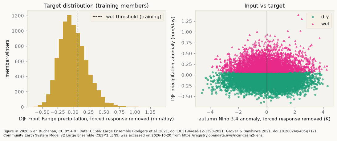
Reading the straight-line relation. NWS Boulder’s sign for east of the Divide is positive — El Niño episodes wetter, La Niña drier — and, for La Niña, the opposite (wetter) for the northwest and north-central mountains, the latter partly in the box’s west column. Its El Niño-wet half is stated “particularly during the late winter and spring of moderate to strong El Niños”, of which DJF holds only February; its La Niña-dry half for southwest and eastern Colorado in “the entire cold season of moderate to strong La Niñas”, while it stresses “the fall and spring of La Niña episodes” for one pattern east of the Divide (the northwest jet). So DJF tests the La Niña-dry half in its stated season and holds only February of the El Niño-wet half. Read the per-member sign count line: do the members share a sign? The standard errors line says whether the mean is distinguishable from zero. Stagge et al. set the observed context: over a climatological model, “the ENSO term explained an additional 2% of total variance” in their regional model, a share of variance across gauges, which they say “should be viewed in the context of extreme spatial and elevation precipitation differences”, and their northern dipole model (“North–Wyoming”) is bounded by 41.2° to 45.5° N. By latitude the Front Range, at about 38.5–40.5° N, falls outside the North–Wyoming model and sits mostly between the poles, its northern edge just past 40° N, though their Fig. 1b shades Colorado’s central mountains, partly in the box’s west column, with the northern pole’s sign; and in the northern pole the sign is reversed, with “increased winter precipitation during La Niña events”.

The wet rate by tenth of the input¶

A correlation sees only a straight line. The cell below prints the wet share in ten equal-count bins of the input, with a binomial standard error and the distance from the base rate in those errors.

show(wet_by_bin)
edges = decile_edges(
    train_tbl
)  # chapter 6 applies these same edges to the test members
bins, chi2, p_chi2, dof = wet_by_bin(train_tbl, edges)
print(
    f"wet rate by decile of the autumn Niño 3.4 anomaly, training members "
    f"(base rate {base_rate:.3f}):"
)
print(bins.round(3).to_string())
print(
    f"chi-square test of wet against decile, training members: "
    f"chi2 = {chi2:.1f}, dof = {dof}, p = {p_chi2:.2g}"
)

wet rate by decile of the autumn Niño 3.4 anomaly, training members (base rate 0.333):
                     wet_rate    n  binomial_se  (rate - base) / se
nino34_anom bin (K)                                                
(-inf, -1.774]          0.270  920        0.015              -4.361
(-1.774, -1.137]        0.342  920        0.016               0.577
(-1.137, -0.726]        0.401  920        0.016               4.191
(-0.726, -0.366]        0.363  920        0.016               1.872
(-0.366, -0.00268]      0.345  920        0.016               0.715
(-0.00268, 0.364]       0.357  920        0.016               1.466
(0.364, 0.738]          0.336  920        0.016               0.161
(0.738, 1.167]          0.309  920        0.015              -1.620
(1.167, 1.743]          0.308  920        0.015              -1.693
(1.743, inf]            0.304  920        0.015              -1.913
chi-square test of wet against decile, training members: chi2 = 51.3, dof = 9, p = 6e-08

The chi-square line says whether the wet rate differs between bins beyond chance. In the table, the coldest bin (the strongest La Niña autumns) and the warmest bins sit below the base rate, the middle above it: a shape no straight line follows. One bin’s departure can be luck; chapter 6 applies these edges to the test members.

The one input, and the ones not chosen¶

One input keeps the model readable whole. Any other field is fair only as an autumn value, known by the start of the winter (at zero lead for a SON mean); NWS Pueblo’s outlook names PNA and NAO as the patterns with the “highest correlations wet/dry”, but as patterns to watch during the winter, which it calls “extremely difficult to forecast more than a few weeks in advance”; whether an autumn value carries into DJF is untested here.

The candidate inputs in the catalogue

Autumn (SON) field	What it stands for	Here
TS over `NINO34`	the ENSO state	the one input (`FEATURES`)
PSL or Z3 over the North Pacific	a stand-in for the autumn PNA state	an untested candidate: whether autumn PNA persists into DJF is not measured here
TREFHT over `FRONT_RANGE`	the box’s own autumn temperature	untested: the box’s state, not the teleconnection
any field averaged over the winter months	the outcome’s own season	never: known only after the outcome
`forcing_variant`	which half a member belongs to	not an input; the per-half check decides pooling

A new input means a new box mean in derive_member_winters and a rebuild, so it is a costed next change, never a quiet edit to FEATURES.

Summary¶

Test members were named first. The forced response came out with a curve fit on training members, checked by a test that can fail. “Wet” is one pooled threshold, so the per-half base rates are a real check. The straight-line relation is weak; the decile table shows a shape a line misses.

What’s next?¶

Chapter 3 builds member-grouped folds and measures what a member-blind split, or transforms fit before it, would do to the score.

Resources and references¶

Resource	Where it bears	Licence
Grover, M., & Banihirwe, A. (2021). NCAR CESM2 Large Ensemble Cloud-Optimized Dataset. NSF NCAR CISL. doi:10.26024/y48t-q717	the dataset (required citation)	UCAR Data Terms of Use
Rodgers, K. B. et al. (2021). Earth System Dynamics 12, 1393–1411. doi:10.5194/esd-12-1393-2021	the ensemble (required citation, with the dataset)	CC BY 4.0
CESM2 Large Ensemble project page. https://www.cesm.ucar.edu/community-projects/lens2	the two forcing halves	UCAR website terms of use
CESM2 LENS intake-esm catalogue (aws-cesm2-le.json). https://ncar-cesm2-lens.s3-us-west-2.amazonaws.com/catalogs/aws-cesm2-le.json	the catalogue search	UCAR Data Terms of Use
scikit-learn User Guide, §12 Common pitfalls and recommended practices; §3.4 Metrics and scoring. https://scikit-learn.org/stable/common_pitfalls.html https://scikit-learn.org/stable/modules/model_evaluation.html	transforms fit on training data only; the base rate	BSD-3-Clause
Stagge, J. H. et al. (2023). Orographic amplification of El Niño teleconnections on winter precipitation across the Intermountain West of North America. Nature Water 1, 1016–1026. doi:10.1038/s44221-023-00163-9	the two poles	CC BY 4.0
NWS Boulder (2020). La Niña and the Upcoming 2020-2021 Winter Season (contains 2010-era slides, e.g. “perhaps through the spring of 2011”). https://www.weather.gov/media/bou/LaNinaWinterOutlook_Sept20.pdf	the expected sign and its season	US Government
NWS Pueblo (2025). Winter of 2025-2026 Outlook. https://www.weather.gov/media/pub/pdf/SC_SE_CO_Winter_2025_26_Outlook.pdf	PNA and NAO	US Government work