Chapter 6’s test is not blind (next section). This chapter runs the test that is left: the same members’ future winters under SSP3-7.0, a period no choice in this cookbook was made on, under a protocol fixed before the scored run (self-attested; no external timestamp).
Overview¶
Why chapter 6’s test is not blind.
The protocol and its decision rule.
Future-period transforms, from the training members only.
The frozen models.
The single scored run, and its reading against the rule.
The limits.
show() prints the source of a lensml.py helper where the chapter uses it.
Prerequisites¶
| Concepts | Importance | Notes |
|---|---|---|
| Chapter 6 | Necessary | the final model, the test and its caveats |
| Chapter 2 | Helpful | the forced response, the wet threshold, the decile bins |
| Distribution shift | Helpful | a model scored on data from another regime than it was fit on |
Time to learn: about 15 minutes; every cell runs in under a minute from the committed caches.
System requirements: the
environment.ymlat the repository root; no account, no local data beyond the committed caches.
Imports¶
import contextlib
import hashlib
import io
import math

import matplotlib.pyplot as plt
import numpy as np
from lensml import (
    FEATURES,
    FUTURE_ACCESS_DATE,
    FUTURE_YEARS,
    RNG_SEED,
    TRIALS,
    apply_transforms,
    at_base_rate,
    cite,
    decile_edges,
    fit_transforms,
    ladder,
    load_future_cache,
    score_frozen,
    setup,
    show,
    show_fig,
    wet_by_bin,
)
Why chapter 6’s test is not blind¶
The 20 test members were scored during development (2026-10-20; the neural network also on 2026-10-29) with the Niño-sign rule, with logistic at the base-rate threshold, which showed no detectable edge, with boosting, the result chapter 6 prints, and in the companion course with a small neural network. Boosting was registered as the final model on 2026-10-29, after those scores had been seen. Every member has been used, so what is left untouched is their future winters: the ssp370 stores, 2016–2100.
The protocol, fixed before the scored run¶
The protocol was written on 2026-10-29, before any SSP3-7.0 data were read, and is followed without change (self-attested; no
external timestamp). It ships verbatim as data/ssp370-test-protocol.md; the hash cell below says whether the file still matches its hash as committed with the test
(851d900; the hash itself was recorded on 2026-10-30). Its decision rule, in its own words:
Primary outcome (decided now): precision − base rate for boosting@base-rate on the test members’ future winters, with the same resampling-over-test-members 95% interval as chapter 6. “Edge replicates” if the interval’s lower bound is above 0; “does not replicate” otherwise. Secondary, reported whatever they show: AP − base rate with interval; recall and wet-call share; false alarms per hit; the same numbers for the comparators; the decile wet rates on the training edges with a chi-square test.
Frozen with it: the model and comparators (always-wet, always-dry, Niño-sign, logistic@base-rate), fitted as in chapter 6 and never refitted. One clarification was made, by the author’s account before the run: “the training edges” are chapter 2’s training-member decile edges (see the sensitivity check below).
How the scoring code was checked
score_frozen, printed below, was checked against chapter 6 (by the author’s account, before the run; the check is not in this
repository, but calling score_frozen on S.test repeats it): on the historical test members it reproduces chapter 6’s
interval lines exactly.
show(score_frozen)PROTOCOL = 'data/ssp370-test-protocol.md'
# The hash of the file as committed with the test (851d900, 2026-10-29),
# recorded here on 2026-10-30: a later edit shows here as 'differs'.
PROTOCOL_SHA256 = (
'11d291795a00bb6d10c818c27a40f9a2a45dff1d8641dfacf931a044489d9628'
)
with open(PROTOCOL, 'rb') as f:
sha = hashlib.sha256(f.read()).hexdigest()
print(f'{PROTOCOL} sha256 {sha} (first 16: {sha[:16]})')
print(
'protocol file: '
+ ('matches' if sha == PROTOCOL_SHA256 else 'DIFFERS from')
+ ' the hash committed with the test'
)data/ssp370-test-protocol.md sha256 11d291795a00bb6d10c818c27a40f9a2a45dff1d8641dfacf931a044489d9628 (first 16: 11d291795a00bb6d)
protocol file: matches the hash committed with the test
The future table¶
data/member_winters_ssp370.csv was derived with chapter 1’s derive_member_winters (same members, boxes and seasons) from the
ssp370 stores, winters 2016–2100; the reader asserts its header. The cell prints only counts.
Why the table starts in 2016
DJF 2015 would need December 2014 from the historical store, so it is dropped.
S = (
    setup()
)  # the historical table: training members, test members, chapter 6's model inputs
fut, fut_header = load_future_cache()
print(fut_header)
fut['split'] = np.where(fut['member_id'].isin(S.test_members), 'test', 'train')
for split, rows in fut.groupby('split'):
    print(
        f'{split}: {rows.member_id.nunique()} members · {len(rows)} future winters'
    )
cache header has no AUTUMN_MONTHS field (it predates the field): taken as AUTUMN_MONTHS=[9, 10, 11], the only autumn the derivation code had: the file's autumn is assumed, not read from the header. A rebuild records it.
# derived by lensml.py: experiment=ssp370 SEASON=DJF WINDOW=(2016, 2100) FRONT_RANGE={'lat': slice(38.5, 40.5, None), 'lon': slice(253.75, 256.25, None)} NINO34={'lat': slice(-5, 5, None), 'lon': slice(190, 240, None)} AUTUMN_MONTHS=[9, 10, 11] n_members=100 RNG_SEED=0 access=2026-10-29
test: 20 members · 1700 future winters
train: 80 members · 6800 future winters
Future-period transforms, from the training members only¶
The forcing differs under SSP3-7.0, so the forced curve and wet threshold are refitted on the training members’ future winters, with chapter 2’s decade check. No test row is read.
fut_train = fut[fut['split'].eq('train')]
TF_FUTURE = fit_transforms(fut_train, years=FUTURE_YEARS)
fut = apply_transforms(fut, TF_FUTURE)
fut_train = fut[fut['split'].eq('train')]
print(
    f"future wet threshold (pooled training members) = {TF_FUTURE['wet_threshold']:+.4f} mm/day; "
    f"training-member future base rate {fut_train['wet'].mean():.3f}"
)
decade = (fut_train['winter'] // 10) * 10
for anom in ['nino34_anom', 'prect_anom']:
    g = fut_train.groupby(decade)[anom]
    z = g.mean() / (fut_train[anom].std() / np.sqrt(g.size()))
    print(
        f"{anom:12s} training members, decade-mean anomaly in standard errors: worst {z[z.abs().idxmax()]:+.2f} "
        f"(the {z.abs().idxmax()}s) · tolerance ±3 → {'PASS' if (z.abs() <= 3).all() else 'FAIL'}"
    )
future wet threshold (pooled training members) = +0.0883 mm/day; training-member future base rate 0.333
nino34_anom  training members, decade-mean anomaly in standard errors: worst +0.85 (the 2050s) · tolerance ±3 → PASS
prect_anom   training members, decade-mean anomaly in standard errors: worst -1.12 (the 2060s) · tolerance ±3 → PASS
# The shift in the input, training members only: no test-member future statistic is computed here.
sd_hist = S.train['nino34_anom'].std()
sd_fut = fut_train['nino34_anom'].std()
print(
    f'SON Niño 3.4 anomaly SD, training members: historical {sd_hist:.3f} K · '
    f'future {sd_fut:.3f} K · ratio {sd_fut / sd_hist:.3f}'
)
SON Niño 3.4 anomaly SD, training members: historical 1.372 K · future 1.538 K · ratio 1.121
The frozen models¶
Each model is fitted once on the 80 training members’ historical winters, as in chapter 6 (the final model is the register’s trial 5). Nothing refits.
X_tr, y_tr = S.train[FEATURES].values, S.train['wet'].values
name5, make5, _ = TRIALS[4]
assert name5 == 'boosting@base-rate'
models = {
    'boosting@base-rate': make5(RNG_SEED).fit(X_tr, y_tr),
    'always-wet': ladder(RNG_SEED)['always-wet'].fit(X_tr, y_tr),
    'always-dry': ladder(RNG_SEED)['always-dry'].fit(X_tr, y_tr),
    'nino-sign': ladder(RNG_SEED)['nino-sign'].fit(X_tr, y_tr),
    'logistic@base-rate': at_base_rate('logistic')(RNG_SEED).fit(X_tr, y_tr),
}
edges = decile_edges(S.train)  # chapter 2's training edges
print('frozen:', ', '.join(models))
frozen: boosting@base-rate, always-wet, always-dry, nino-sign, logistic@base-rate
The scored run¶
This cell is the test: the primary outcome, then the secondary outcomes in the protocol’s order, then the decile chi-square. A counter marks any re-run in the same kernel, and the cell after it compares the result with the first scored run, so a library upgrade that changed it shows as “differs”.
SCORED_RUNS = globals().get('SCORED_RUNS', 0) + 1
print(
    f'scored run #{SCORED_RUNS}'
    + ('' if SCORED_RUNS == 1 else '   — a re-run in this kernel')
)
fut_test = fut[fut['split'].eq('test')].reset_index(drop=True)
buf = io.StringIO()
with contextlib.redirect_stdout(buf):
    results = score_frozen(models, fut_test, edges)
pt, lo, hi = results['boosting@base-rate']['precision − base rate']
verdict = 'EDGE REPLICATES' if lo > 0 else 'DOES NOT REPLICATE'
print(
    f"PRIMARY OUTCOME — boosting@base-rate, precision − base rate on the test members' future winters: {pt:+.3f}, "
    f'95% interval over test members [{lo:+.3f}, {hi:+.3f}] → {verdict} '
    '(pre-registered rule: replicates only if the lower bound is above 0)'
)
print('\nSECONDARY OUTCOMES, in the protocol\'s order:')
print(buf.getvalue())
scored run #1
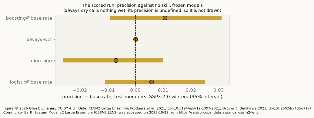
PRIMARY OUTCOME — boosting@base-rate, precision − base rate on the test members' future winters: +0.011, 95% interval over test members [-0.009, +0.031] → DOES NOT REPLICATE (pre-registered rule: replicates only if the lower bound is above 0)

SECONDARY OUTCOMES, in the protocol's order:
20 members · 1700 winters · base rate 0.317
boosting@base-rate: precision − base rate  +0.011   95% interval over members [-0.009, +0.031]  →  NOT distinguishable from no skill
boosting@base-rate: AP − base rate         +0.014   95% interval over members [-0.003, +0.038]  →  NOT distinguishable from no skill
boosting@base-rate: recall 0.570  wet-call share 0.551  false alarms 630 · hits 307 · false alarms per hit 2.05
always-wet: precision − base rate  +0.000   95% interval over members [+0.000, +0.000]  →  NOT distinguishable from no skill
always-wet: AP − base rate         +0.000   95% interval over members [+0.000, +0.000]  →  NOT distinguishable from no skill
always-wet: recall 1.000  wet-call share 1.000  false alarms 1161 · hits 539 · false alarms per hit 2.15
always-dry: precision − base rate  -0.317   95% interval over members [-0.337, -0.295]  →  below no skill
always-dry: AP − base rate         +0.000   95% interval over members [+0.000, +0.000]  →  NOT distinguishable from no skill
always-dry: recall 0.000  wet-call share 0.000  false alarms 0 · hits 0 · false alarms per hit undefined (no hits)
nino-sign: precision − base rate  -0.007   95% interval over members [-0.026, +0.010]  →  NOT distinguishable from no skill
nino-sign: AP − base rate         -0.003   95% interval over members [-0.012, +0.005]  →  NOT distinguishable from no skill
nino-sign: recall 0.484  wet-call share 0.495  false alarms 581 · hits 261 · false alarms per hit 2.23
logistic@base-rate: precision − base rate  +0.006   95% interval over members [-0.011, +0.025]  →  NOT distinguishable from no skill
logistic@base-rate: AP − base rate         -0.010   95% interval over members [-0.025, +0.013]  →  NOT distinguishable from no skill
logistic@base-rate: recall 0.516  wet-call share 0.506  false alarms 583 · hits 278 · false alarms per hit 2.10
wet rate by bin of the autumn Niño 3.4 anomaly (edges given):
                     wet_rate    n  binomial_se  (rate - base) / se
nino34_anom bin (K)
(-inf, -1.774]          0.252  230        0.029              -2.266
(-1.774, -1.137]        0.372  172        0.037               1.493
(-1.137, -0.726]        0.354  147        0.039               0.930
(-0.726, -0.366]        0.350  157        0.038               0.874
(-0.366, -0.00268]      0.322  152        0.038               0.140
(-0.00268, 0.364]       0.285  151        0.037              -0.879
(0.364, 0.738]          0.326  141        0.039               0.233
(0.738, 1.167]          0.339  165        0.037               0.606
(1.167, 1.743]          0.291  165        0.035              -0.740
(1.743, inf]            0.309  220        0.031              -0.256
chi-square test of wet against bin: chi2 = 10.4, dof = 9, p = 0.32
# The first scored run, as the author recorded it on 2026-10-29 (first
# committed 2026-10-30). A library upgrade that changes the scored result
# shows here as 'differs'; report a changed result as a re-run.
FIRST_RUN = (0.011, -0.009, 0.031, 'DOES NOT REPLICATE')
now = (round(pt, 3), round(lo, 3), round(hi, 3), verdict)
print(
    'scored result: '
    + ('matches' if now == FIRST_RUN else f'DIFFERS from {FIRST_RUN}:')
    + (' the first scored run' if now == FIRST_RUN else f' now {now}')
)
scored result: matches the first scored run
# Chapter 6's estimate, recomputed from the historical test members (already scored there), against this interval.
yhat_hist = models['boosting@base-rate'].predict(S.test[FEATURES].values)
w_hist = S.test['wet'].values
est6 = w_hist[yhat_hist == 1].mean() - w_hist.mean()
print(
    f"chapter 6's estimate (historical test members) {est6:+.3f}; inside this "
    f'interval [{lo:+.3f}, {hi:+.3f}]: {lo <= round(est6, 3) <= hi}'
)
# Outside the protocol: how often a test this size would confirm an edge of
# chapter 6's size (a normal approximation to the interval over members).
se7 = (hi - lo) / (2 * 1.96)
power7 = 0.5 * (1 - math.erf((1.96 - est6 / se7) / math.sqrt(2)))
print(
    f'outside the protocol: with this interval\'s width (SE ≈ {se7:.4f}), '
    f"a true edge of chapter 6's size clears a lower bound of 0 about "
    f'{power7:.0%} of the time'
)
chapter 6's estimate (historical test members) +0.018; inside this interval [-0.009, +0.031]: True
outside the protocol: with this interval's width (SE ≈ 0.0102), a true edge of chapter 6's size clears a lower bound of 0 about 42% of the time
names = [
    n for n in results if n != 'always-dry'
]  # undefined precision, not drawn
fig, ax = plt.subplots(figsize=(7, 3.2))
for i, name in enumerate(names):
    p, a, b = results[name]['precision − base rate']
    ax.plot([a, b], [i, i], color='#C9A23A', lw=9, solid_capstyle='butt')
    ax.plot(
        p, i, 'o', color='#8F7022', markeredgecolor='#13161A', markersize=9
    )
ax.axvline(0, color='#13161A', ls='--', lw=1)
ax.set_yticks(range(len(names)), names)
ax.invert_yaxis()
ax.set_xlabel(
    'precision − base rate, test members\' SSP3-7.0 winters (95% interval)'
)
ax.set_title(
    'The scored run: precision against no skill, frozen models\n'
    '(always-dry calls nothing wet: its precision is undefined, so it is not drawn)',
    fontsize=9,
)
cite(fig, FUTURE_ACCESS_DATE)  # the ssp370 table's access date
plt.tight_layout()
show_fig(
    fig,
    (
        "Horizontal interval plot: for each frozen model — boosting at "
        "the base-rate threshold, always-wet, the Niño-sign rule and "
        "logistic at the base-rate threshold — a dot for precision minus "
        "the base rate on the test members' SSP3-7.0 winters and a gold "
        "bar for its 95% interval over test members, against a dashed "
        "line at zero, no skill. Always-dry is not drawn: it calls "
        "nothing wet, so its precision is undefined."
    ),
)
Reading the run against the rule¶
The edge does not replicate under the rule fixed, by the author’s account, before the run. On the PRIMARY OUTCOME line, the final model’s precision
interval includes zero. The chapter 6's estimate line shows it also includes chapter 6’s estimate, so this test cannot separate no
edge from an edge of that size; the outside the protocol line shows how small the test was. It
gives no support for a briefing calling the winter statistically wetter.
The secondary outcomes agree: the final model’s AP − base rate line is not distinguishable from no skill, no comparator clears the
base rate on precision, and every model that calls wet makes more false alarms than hits (the false alarms per hit values).
Always-dry calls nothing wet, so its precision is undefined: the scored-run line reads “below no skill” only because
precision is scored 0 when nothing is called wet (it is not drawn in the figure). The decile chi-square line does not reject chance.
This does not show the historical edge was an artefact (a shift could hide a real but fragile relation, limit 1), but the chapter 6 edge is not evidence a forecaster could lean on.
A choice the protocol left open: the bin edges¶
The protocol did not say which period’s “training edges”; the run used chapter 2’s historical ones (the clarification above, by the
author’s account made before the run). The cell below tries the future-winter edges, outside the protocol: the two p values
differ and neither rejects chance at 0.05.
# Sensitivity, outside the protocol: the decile chi-square on the test
# members' future winters under each reading of "the training edges".
for label, e in [
    ("chapter 2's historical training edges (the run)", edges),
    ("the training members' future-winter edges", decile_edges(fut_train)),
]:
    _, chi2, p, dof = wet_by_bin(fut_test, e)
    print(f'{label}: chi2 {chi2:.1f}, dof {dof}, p {p:.2f}')
chapter 2's historical training edges (the run): chi2 10.4, dof 9, p 0.32
the training members' future-winter edges: chi2 11.9, dof 9, p 0.22
Limits¶
A different period under stronger forcing. A failure can be shift as well as no skill: the model was fit on 1900–2014 and scored on 2016–2100, and the input is wider (the
SON Niño 3.4 anomaly SDline). Rodgers et al. (2021) find “a decrease in ENSO amplitude” in the Niño 3.4 region and “decreased precipitation co-variance with ENSO” over the Pacific Northwest and much of the southern US and Mexico under the same forcing; this SON box mean moves the other way (the SD line prints a wider input), though they compare DJF 1960–1989 with 2070–2099 while this pools 2016–2100 against 1900–2014; the two are not reconciled here. Either way, this test asks whether the edge holds under a changed relation as much as whether it was real.A model world. CESM2 scored against CESM2; nothing here touches observations.
The same members. The 20 test members were scored during development; their future winters are new data, and the target shows little year-to-year memory (chapter 3’s lag-1 line); what carries over is that these members took part in choosing the model.
The existing limits. Chapter 6’s limits 2–7 hold unchanged.
Chapter 6’s limits 2–7, listed
CESM2’s own ENSO and teleconnection, a ~1° grid, DJF, which holds only February of the late winter and spring NWS Boulder stresses for El Niño east of the Divide, total precipitation, one forced curve for both halves, a box that crosses the Divide.
Summary¶
A protocol fixed the model, outcomes and decision rule before any SSP3-7.0 data were read (self-attested); the frozen models were scored once. The
edge does not replicate under the rule fixed before the run (the PRIMARY OUTCOME line), and the interval also includes chapter 6’s
estimate.
What’s next?¶
The same protocol could be run in another season (FMA), another box or another ensemble, each written down before its data are read. Observed winters remain the test that would tell a model result from a real one.
Resources and references¶
| Resource | Where it bears | Licence |
|---|---|---|
| Grover, M., & Banihirwe, A. (2021). NCAR CESM2 Large Ensemble Cloud-Optimized Dataset. NSF NCAR CISL. doi:10.26024/y48t-q717 | the ssp370 stores (required citation) | UCAR Data Terms of Use |
| Rodgers, K. B. et al. (2021). Earth System Dynamics 12, 1393–1411. doi:10.5194/esd-12-1393-2021 | the ensemble and its SSP3-7.0 forcing (required citation); limit 1 | CC BY 4.0 |
| scikit-learn User Guide, §12 Common pitfalls. https:// | transforms fit on training data only | BSD-3-Clause |
Results based on the CESM2 Large Ensemble acknowledge the CESM2 Large Ensemble Community Project and supercomputing resources provided by the IBS Center for Climate Physics in South Korea.